What are we modeling? Using predictive fit to inform effect metric choice in meta-analysis

James E. Pustejovsky

2025-10-09

Research Synthesis

The systematic integration of empirical results across multiple sources of evidence, for purposes of drawing generalizations¹.

Meta-Analysis

Statistical models and methods to support quantitative research synthesis.

Fields that rely on research synthesis

• Medicine (Cochrane Collaboration)
• Education (What Works Clearinghouse)
• Psychology
• Social policy (justice, welfare, public health, etc.)
• Economics, international development
• Ecology and Environmental Science
• Physical sciences

• Some background on meta-analysis

• The problem of effect metric choice

• Proposal: Use predictive fit criteria to inform metric choice

• Illustrations

• Discussion

Canonical Meta-Analysis

• We observe summary results from each of \(k\) studies:

  • \(T_i\) - effect size estimate

  • \(se_i\) - standard error of effect size estimate

  • \(N_i\), \(\mathbf{x}_i\) - sample size, other study features

• A summary random effects model: \[ \begin{aligned} T_i &\sim N\left(\theta_i, \ se_i^2 \right) \\ \theta_i &\sim N\left(\mu, \ \tau^2\right) \end{aligned} \]

• A random effects meta-regression: \[ \begin{aligned} T_i &\sim N\left(\theta_i, \ se_i^2 \right) \\ \theta_i &\sim N\left(\mathbf{x}_i \boldsymbol\beta,\ \tau^2\right) \end{aligned} \]

• “Conceptual unity of statistical methods” for meta-analysis² suggests that most any effect size measure \(\theta_i\) can be used, as long as \(T_i \dot{\sim} N\left(\theta_i, \ se_i^2 \right)\).

Prediction Interval

• An approximate \(1 - 2\alpha\) prediction interval for a new study-specific parameter \(\theta_{new}\)³:

  \[ \hat\mu \ \pm \ q_\alpha \times\sqrt{\hat\tau^2 + \mathbb{V}\left(\hat\mu\right)} \]

  • Largely used to characterize the extent of effect heterogeneity⁴.

• Beyond this, “predictive modeling” culture^5,6 seems to have very little influence on meta-analysis.

Effect Metric Menagerie

Effect Metric Families

Single-group summaries

• Raw proportions \(\pi\)
• Arcsine-transformation \(a = \text{asin}\left(\sqrt{\pi}\right)\)
• Raw means \(\mu\)

Bivariate associations / psychometric

• Pearson’s correlation \(\rho\)
• Fisher’s \(z\)-transformation \(\zeta = \text{atanh}(\rho)\)
• Cronbach’s \(\alpha\) coefficients (or transformations thereof)

Group comparison of binary outcomes

• Risk differences \(\pi_1 - \pi_0\)
• Risk ratios (log-transformed) \(\log\left(\frac{\pi_1}{\pi_0}\right)\)
• Odds ratios (log-transformed) \(\log\left(\frac{\pi_1 / (1 - \pi_1)}{\pi_0 / (1 - \pi_0)}\right)\)
• Bivariate models for \(\pi_0, \pi_1\)

Group comparison of continuous outcomes

• Raw mean differences \(\mu_1 - \mu_0\)
• Standardized mean differences \(\delta = \frac{\mu_1 - \mu_0}{\sigma}\)
• Response ratios (log-transformed) \(\lambda = \log\left(\frac{\mu_1}{\mu_0}\right)\)
• Probability of superiority

Metric choice methodology

• Large literature on effect metrics for group comparison on binary outcomes.

  • Theoretical arguments about interpretability, stability, non-collapsibility^7,8.

  • Risk differences tend to be more heterogeneous^9,10.

• Strong opinions about effect metrics for group comparison on continuous outcomes¹¹.

  • Some novel alternatives to avoid standarization^12–14.

  • Various methods for standardization^{e.g., 15,16}.

• Choice between standardized mean difference and response ratio metrics

  • Sensitivity analyses using both metrics¹⁷.

  • Model both metrics simultaneously¹⁸.

Effect Metric Choice

• Choice of metric is constrained by

  • Studies designs

  • Data availability, reporting conventions

  • Heterogeneity of study features (e.g., outcome scales)

• Metric choice is driven by disciplinary conventions.

  • In many applications, more than one metric could apply.

Metric choice by predictive fit criteria

• Evaluate effect metrics by performance in predicting summary data for a new study.

  • Data vector \(\mathbf{d}_i\) consisting of summary statistics used to compute effect size estimates.

• Use leave-one-out log-predictive density to measure predictive performance. \[ LPD = \frac{1}{k} \sum_{i=1}^{k} \log p\left(\mathbf{d}_i \left| \hat\mu_{(-i)}, \hat\tau_{(-i)}, \mathbf{X}_i, N_i\right.\right) \]

Two challenges

1. Polishing up models to generate predictions.

2. Conventional meta-analysis focuses on one-dimensional \(f(\mathbf{d}_i)\), so we need auxiliary models for the rest of the data.

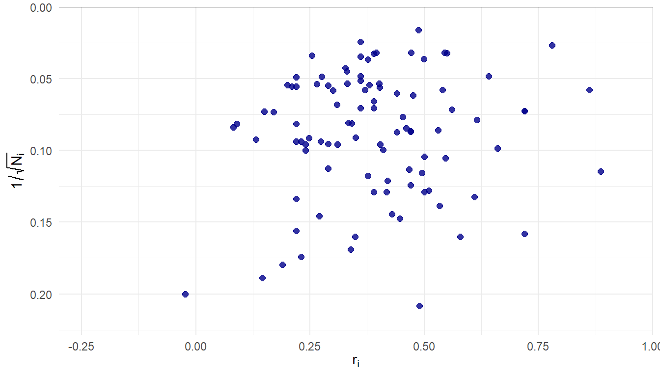
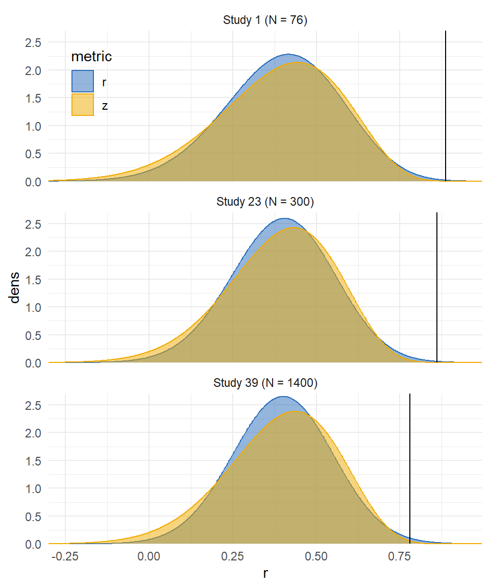
Class attendance and college grades

• Credé and colleagues¹⁹ reported a systematic review and meta-analysis of studies on association between class attendance and grades / GPA in college.

• 99 correlation estimates, samples ranging from \(N_i\) = 23 to 3900 (median = 151, IQR = 76-335).

Bivariate associations

• The data: Pearson correlation between two variables of interest from a sample of \(N_i\) observations, \(r_i\).

\(\rho\) metric

• Effect size estimate \(r_i\), standard error \(\displaystyle{se_i = \frac{1 - r_i^2}{\sqrt{N_i}}}\)

• Predictive model: \[ \begin{aligned} r_i &\dot{\sim} \ N\left(\rho_i, \ \frac{(1 - \rho_i^2)^2}{N_i}\right) \\ \rho_i &\sim \ N_{trunc}\left(\mu_\rho, \ \tau_\rho^2\right) \end{aligned} \]

\(\zeta = \text{atanh}(\rho)\) metric

• Effect size estimate \(z_i = \text{atanh}(r_i)\), standard error \(\displaystyle{se_i = \frac{1}{\sqrt{N_i - 3}}}\)

• Predictive model: \[ \begin{aligned} z_i &\dot{\sim} \ N\left(\zeta_i, \ \frac{1}{N_i - 3}\right) \\ \zeta_i &\sim \ N\left(\mu_\zeta, \ \tau_\zeta^2\right) \end{aligned} \]

• log-predictive density: \[\begin{eqnarray} \log &d_r&(r_i | \hat\mu_{\zeta (-i)}, \hat\tau_{\zeta (-i)}, N_i) \\ &=& \log d_z\left(z_i \left| \hat\mu_{\zeta (-i)}, \hat\tau_{\zeta (-i)}, N_i \right.\right) - \log\left(1 - r_i^2\right) \end{eqnarray}\]

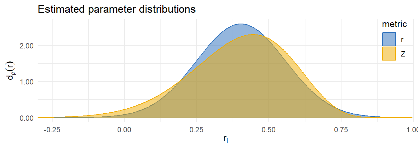
Metric comparison

Metric	Est.	95% CI	80% PI	LPD	SE
r	0.40	0.37-0.44	0.20-0.60	0.34	0.09
z	0.41	0.37-0.45	0.16-0.61	0.22	0.12
Difference				0.12	0.05

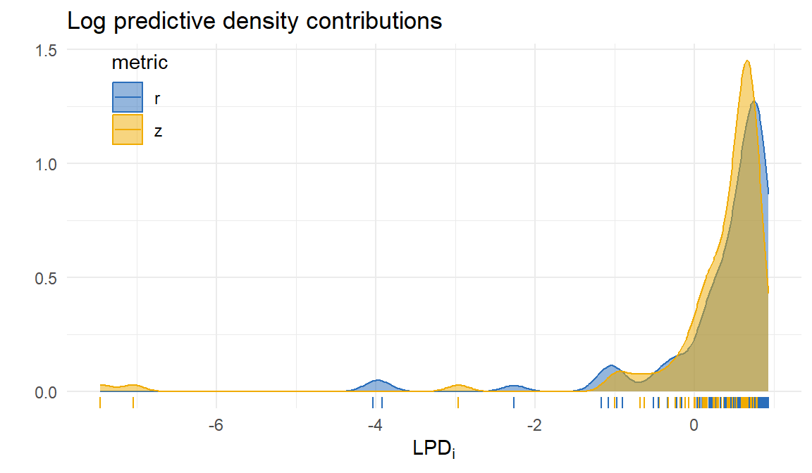
Outliers

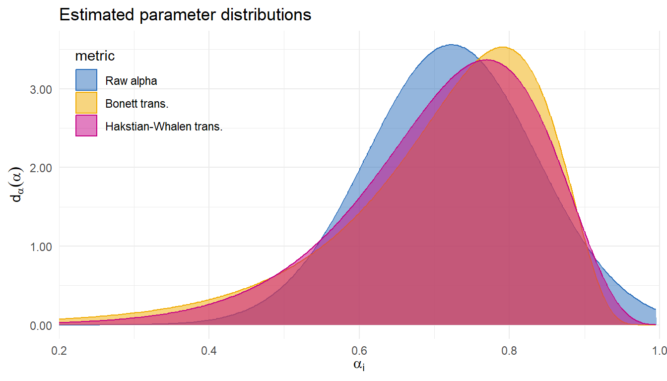
Reliability generalization of MIBS

• Demir and colleagues²⁰ gathered 33 estimates of internal consistency (Cronbach \(\alpha\)) of the Mother-to-Infant Bonding Scale.

• Sample sizes ranging from \(N_i\) = 13 to 2251 (median = 177, IQR = 98-260).

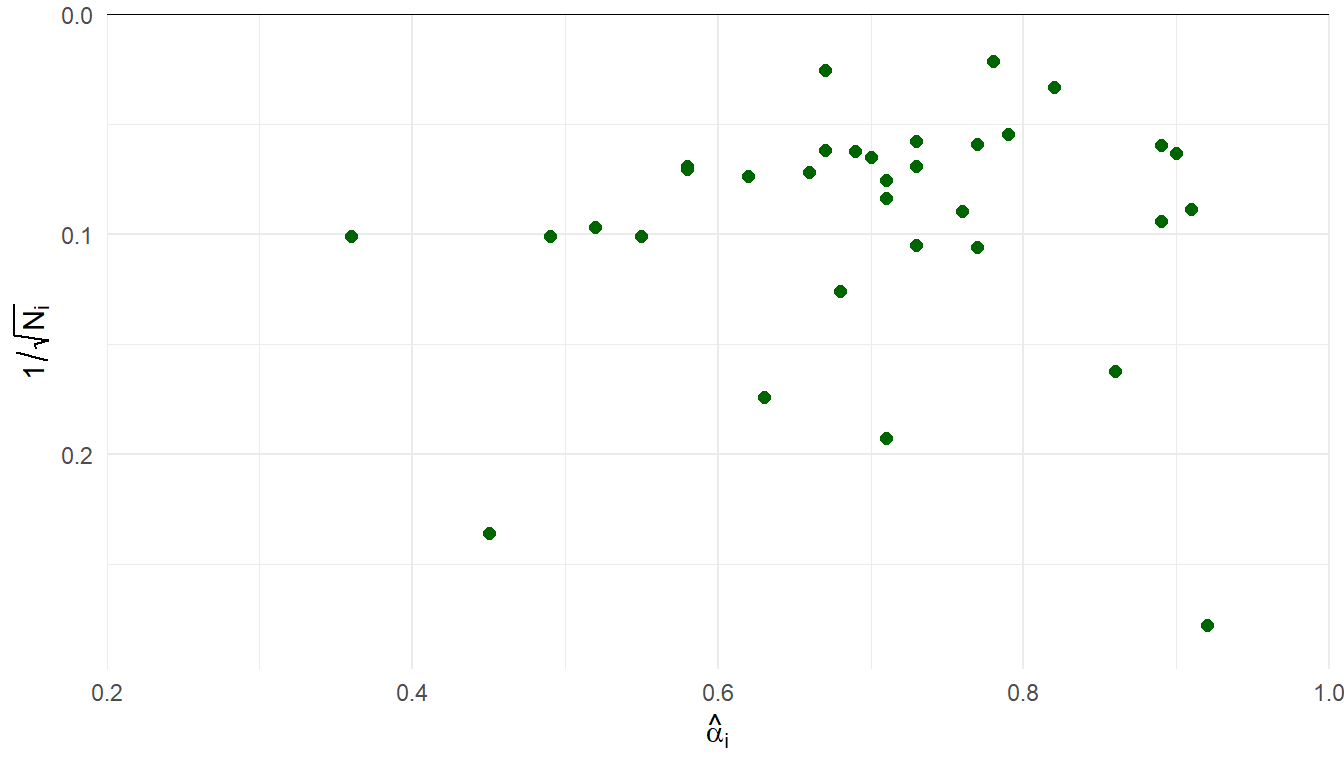
Metric	Est.	95% CI	80% PI	LPD	SE
Raw alpha	0.72	0.68-0.76	0.58-0.87	0.57	0.16
Bonett trans.	0.74	0.69-0.78	0.51-0.86	0.53	0.12
Hakstian-Whalen trans.	0.73	0.68-0.77	0.53-0.86	0.58	0.11

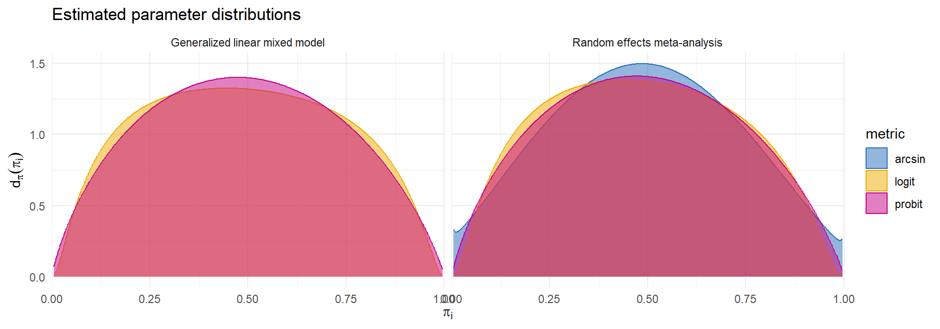
Incidence of olfactory loss in COVID-19 patients

• Hannum and colleagues²¹ compiled data on rates of olfactory loss across 35 studies of COVID-19 patients.

• Sample sizes ranging from \(N_i\) = 15 to 7178 (median = 95, IQR = 56.5 - 267.5).

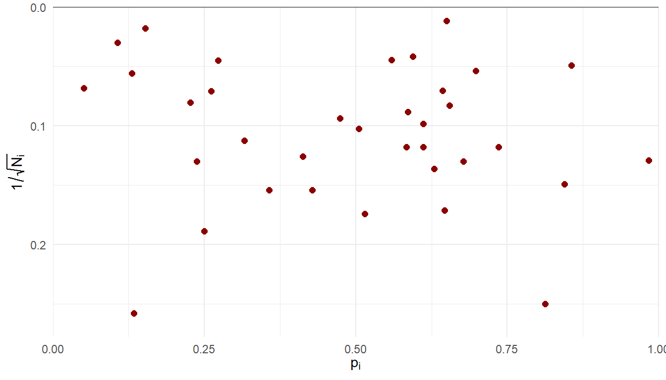
• Many different transformations of \(p_i\) are used as effect size measures (identity, logit, probit, arcsin-square-root, Freeman-Tukey).

• Could use conventional random effects model or generalized linear mixed model.

• Which predictive model to use?

\[ \begin{aligned} g(p_i) &\dot{\sim} \ N\left(g(\pi_i), \ \frac{h(\pi_i)}{N_i}\right) \qquad & N_i p_i &\sim \ Binom\left(N_i, \ \pi_i\right)\\ g(\pi_i) &\sim \ N\left(\mu_g, \ \tau_g^2\right) \qquad & g(\pi_i) &\sim \ N\left(\mu_g, \ \tau_g^2\right) \end{aligned} \]

Incidence of olfactory loss in COVID-19 patients

					Normal		Binomial
Model	Metric	Est.	95% CI	80% PI	LPD	SE	LPD	SE
RE	logit	0.48	0.38-0.58	0.17-0.81	-5.10	0.36	-5.11	0.36
RE	probit	0.49	0.39-0.58	0.17-0.81	-5.18	0.40	-5.18	0.40
RE	arcsin	0.49	0.40-0.58	0.17-0.81	-4.96	0.32	-4.96	0.32
GLMM	logit	0.48	0.38-0.59	0.16-0.82			-5.43	0.55
GLMM	probit	0.49	0.39-0.58	0.17-0.82			-5.24	0.43

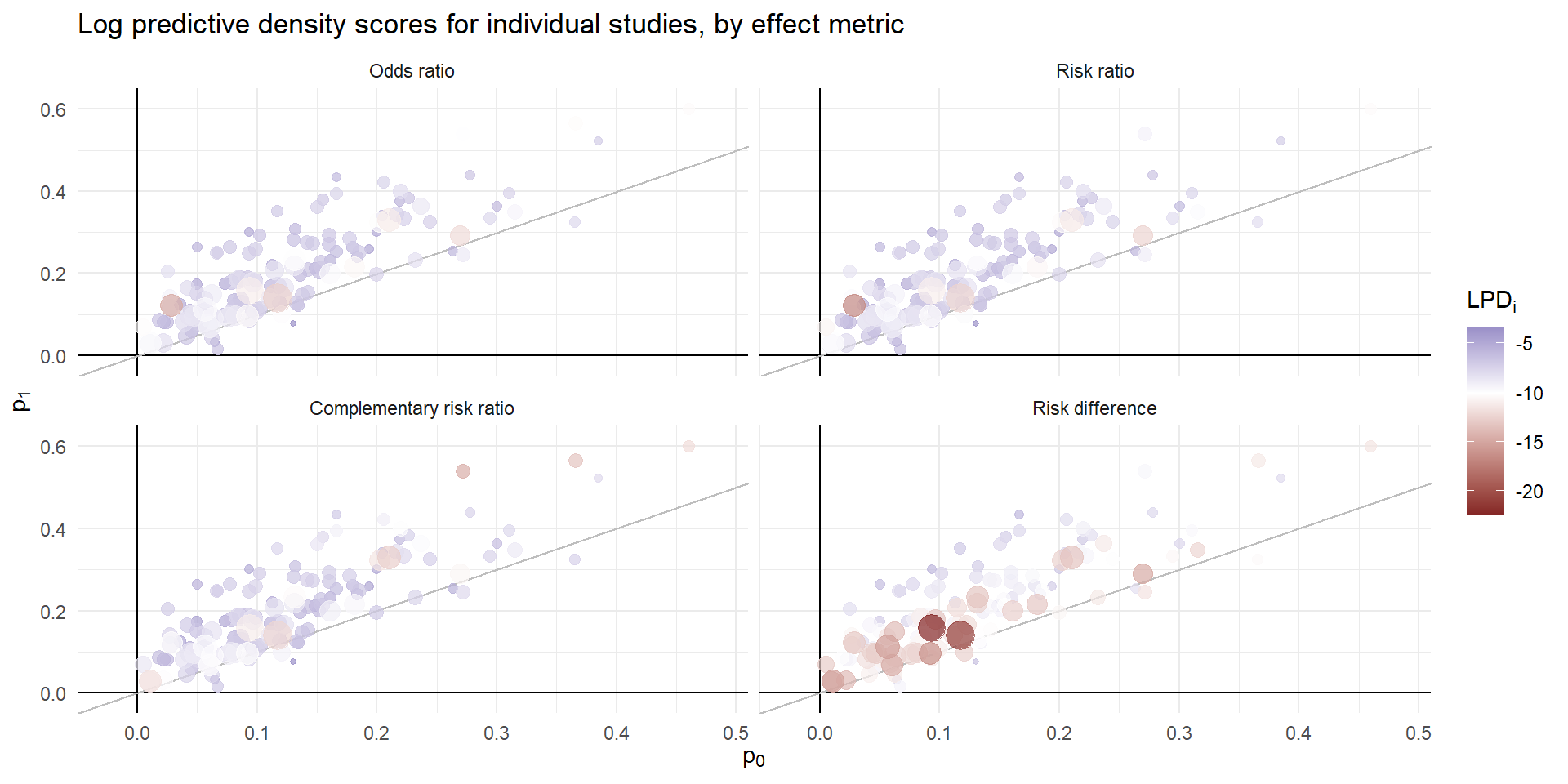
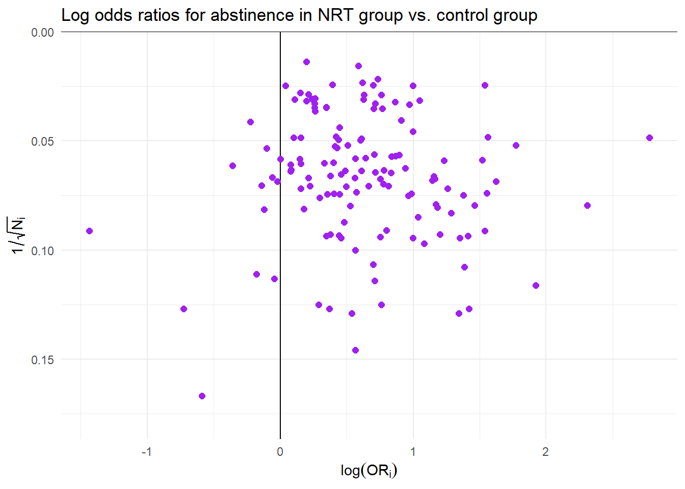
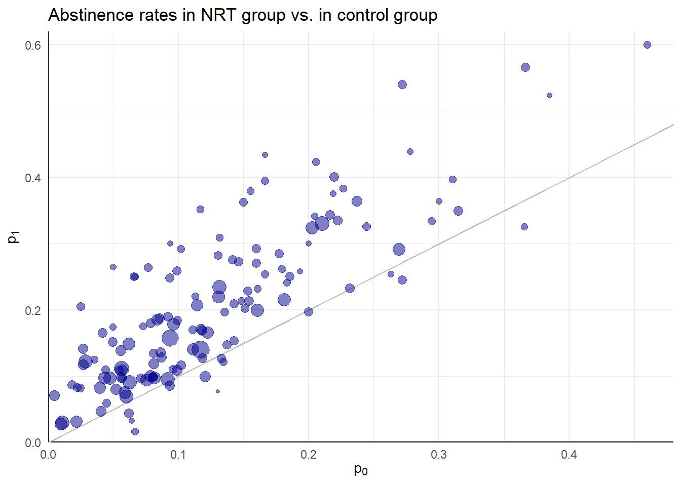
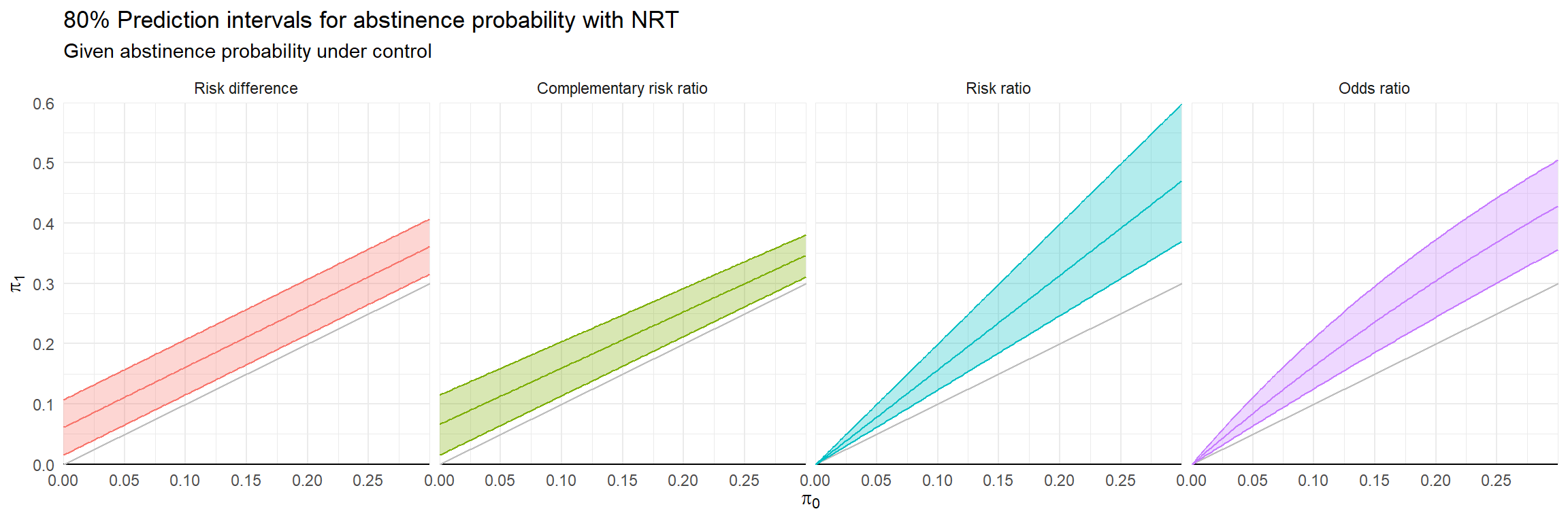
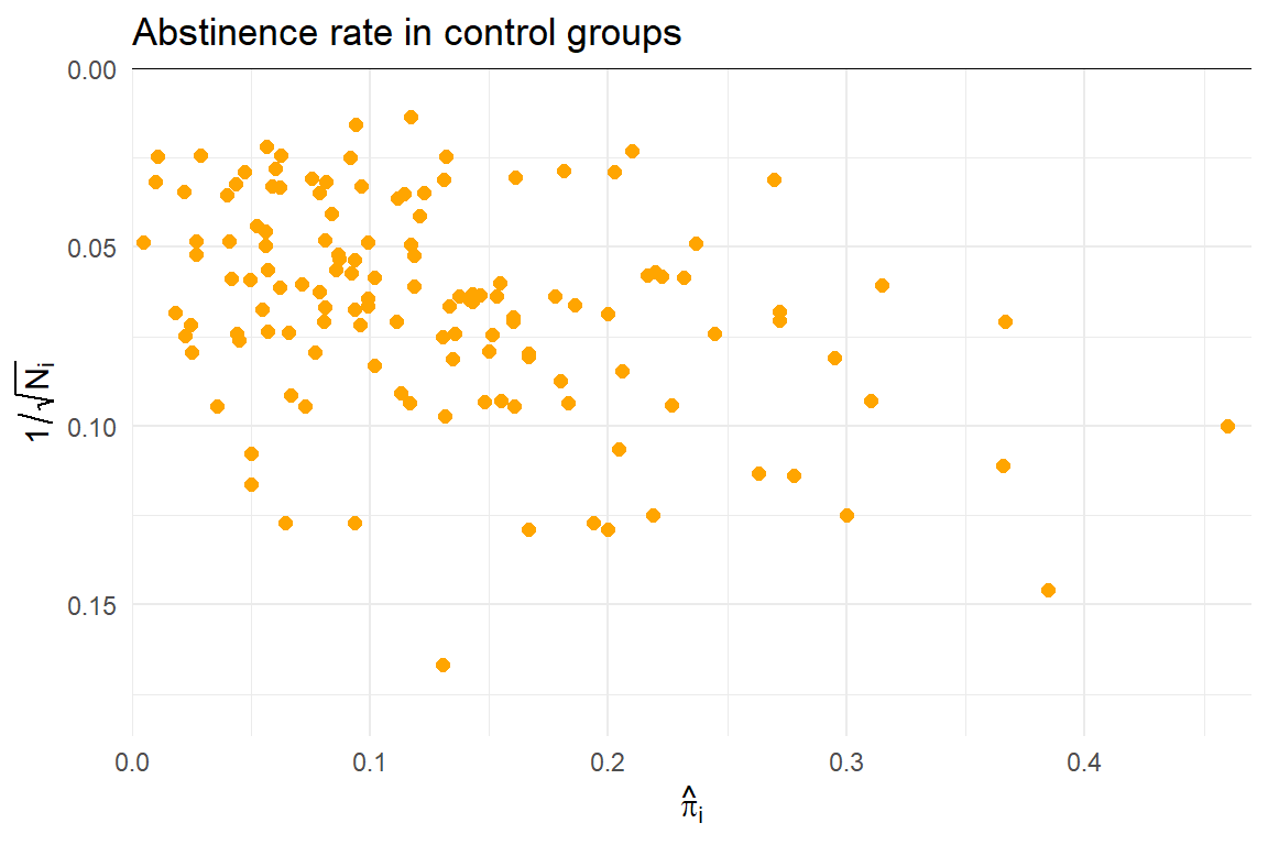
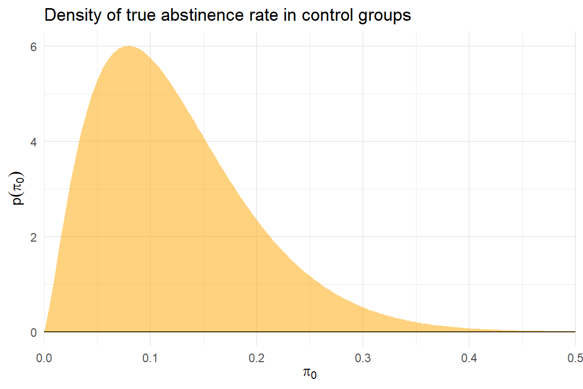
Effectiveness of nicotine replacement therapy

• Cochrane Systematic Review of effects of nicotine replacement therapy vs. control on smoking cessation, defined as abstinence at 6+ month follow-up²².

• Sample sizes ranging from \(N_i\) = 36 to 5290 (median = 240.5, IQR = 153.5 - 428.5).

• Multiple possible effect metrics: log odds ratio, log risk ratio, complementary log risk ratio, risk difference

• Alternative models: bivariate meta-analysis²³, bivariate logistic or hypergeometric GLMM²⁴, baseline risk regression^25–27, etc.

Random effects meta-analysis

• Difference ES metrics suggest very different implications and different heterogeneity

Metric	Est	95% CI	80% PI	I2
Risk difference	0.06	0.05-0.07	0.02-0.11	63.50
Complementary risk ratio	1.07	1.06-1.08	1.02-1.13	65.51
Risk ratio	1.57	1.48-1.66	1.23-1.99	36.88
Odds ratio	1.75	1.63-1.88	1.29-2.38	39.06

Effect metric comparison

• Goal: evaluate predictions of \(\hat\pi_{0i}\), \(\hat\pi_{1i}\) using log-predictive density.

• Conventional RE meta-analysis is a model for \(f(\hat\pi_{0i}, \hat\pi_{1i})\).

• Possible auxiliary models for \(\hat\pi_{0i}\) or \(\hat\pi_{1i}\):

  • Random effects meta-analysis/meta-regression

  • Generalized linear mixed model

  • Beta-binomial regression

Predictive model

\[ \begin{aligned} &\text{Auxiliary model:} \quad & \pi_{0i} &\sim Beta\left(\alpha, \ \beta\right) \\ &\text{RE meta-analysis model:} \quad & \theta_i &\sim N\left(\mu, \ \tau^2\right) \\ &\text{Observation model:} \quad & N_{0i} \hat\pi_{0i} &\sim Binom\left( N_{0i}, \ \pi_{0i} \right) \\ & & N_{1i} \hat\pi_{1i} &\sim Binom\left( N_{0i}, \ g(\pi_{0i}, \theta) \right) \end{aligned} \]

Metric comparison

Metric	LPD	SE	Diff. vs. OR	SE
Odds ratio	-7.300	0.151
Risk ratio	-7.342	0.157	-0.041	0.019
Complementary risk ratio	-7.443	0.163	-0.143	0.076
Risk difference	-10.152	0.217	-2.852	0.135

Predictive discrepancies

Discussion

• Effect metric choice is a modeling assumption.

• Predictive fit assessment is relevant and useful for meta-analysis.

  • Log predictive density calculations should be part of meta-analysts’ toolkit.

  • Will often require use of auxiliary models.

• Advantages of log predictive density scoring

  • Allows comparison across effect metrics and different forms of models.

  • Auxiliary model building exercise can clarify scientific context.

• Disadvantages and open questions

  • Deshpande and colleagues²⁸ highlight discrepancies between LPD and other model evaluation metrics.

  • Other predictive scoring rules that may be relevant?

  • Is the joint distribution of \(\mathbf{d}_i\) the right focus?

References

1.

Cooper, H. & Hedges, L. V. Research synthesis as a scientific enterprise. in The Handbook of Research Synthesis and Meta-Analysis (eds. Cooper, H., Hedges, L. V. & Valentine, J. C.) 3–14 (Russell Sage Foundation, New York, NY, 2009).

2.

Hedges, L. V. Statistical considerations. in The Handbook of Research Synthesis and Meta-Analysis (eds. Cooper, H., Hedges, L. V. & Valentine, J. C.) 37–48 (Russell Sage Foundation, New York, NY, 2019).

3.

Higgins, J. P. T., Thompson, S. G. & Spiegelhalter, D. J. A re-evaluation of random-effects meta-analysis. Journal of the Royal Statistical Society: Series A (Statistics in Society) 172, 137–159 (2009).

4.

Borenstein, M., Higgins, J. P. T., Hedges, L. V. & Rothstein, H. R. Basics of meta-analysis: I ² is not an absolute measure of heterogeneity. Research Synthesis Methods 8, 5–18 (2017).

5.

Breiman, L. Statistical modeling: The two cultures. Statist. Sci. 16, (2001).

6.

Donoho, D. 50 years of data science. Journal of Computational and Graphical Statistics 26, 745–766 (2017).

7.

Poole, C., Shrier, I. & VanderWeele, T. J. Is the risk difference really a more heterogeneous measure? Epidemiology 26, 714 (2015).

8.

Panagiotou, O. A. & Trikalinos, T. A. Commentary: On effect measures, heterogeneity, and the laws of nature. Epidemiology 26, 710 (2015).

9.

Engels, E. A., Schmid, C. H., Terrin, N., Olkin, I. & Lau, J. Heterogeneity and statistical significance in meta-analysis: An empirical study of 125 meta-analyses. Statist. Med. 19, 1707–1728 (2000).

10.

Zhao, Y., Slate, E. H., Xu, C., Chu, H. & Lin, L. Empirical comparisons of heterogeneity magnitudes of the risk difference, relative risk, and odds ratio. Syst Rev 11, 26 (2022).

11.

Cummings, P. Arguments for and against standardized mean differences (effect sizes). Arch Pediatr Adolesc Med 165, 592–596 (2011).

12.

Ades, A. E., Lu, G., Dias, S., Mayo-Wilson, E. & Kounali, D. Simultaneous synthesis of treatment effects and mapping to a common scale: An alternative to standardisation. Research Synthesis Methods 6, 96–107 (2015).

13.

Lu, G., Kounali, D. & Ades, A. E. Simultaneous multioutcome synthesis and mapping of treatment effects to a common scale. Value Health 17, 280–287 (2014).

14.

Davies, A. L., Ades, A. E. & Higgins, J. P. T. Mapping between measurement scales in meta-analysis, with application to measures of body mass index in children. Research Synthesis Methods 15, 1072–1093 (2024).

15.

Hopkins, W. G. & Rowlands, D. S. Standardization and other approaches to meta-analyze differences in means. Statistics in Medicine 43, 3092–3108 (2024).

16.

Fitzgerald, K. G. & Tipton, E. Using extant data to improve estimation of the standardized mean difference. Journal of Educational and Behavioral Statistics 50, 128–148 (2025).

17.

Friedrich, J. O., Adhikari, N. K. J. & Beyene, J. Ratio of means for analyzing continuous outcomes in meta-analysis performed as well as mean difference methods. J Clin Epidemiol 64, 556–564 (2011).

18.

Yang, Y. et al. Bivariate multilevel meta-analysis of log response ratio and standardized mean difference for robust and reproducible environmental and biological sciences. 2024.05.13.594019 https://www.biorxiv.org/content/10.1101/2024.05.13.594019v1 (2024).

19.

Credé, M., Roch, S. G. & Kieszczynka, U. M. Class attendance in college: A meta-analytic review of the relationship of class attendance with grades and student characteristics. Review of Educational Research 80, 272–295 (2010).

20.

Demir, E., Öz, S., Aral, N. & Gürsoy, F. A reliability generalization meta-analysis of the Mother-To-Infant Bonding Scale. Psychol Rep 127, 447–464 (2024).

21.

Hannum, M. E. et al. Objective sensory testing methods reveal a higher prevalence of olfactory loss in COVID-19–positive patients compared to subjective methods: A systematic review and meta-analysis. Chemical Senses bjaa064 (2020) doi:10.1093/chemse/bjaa064.

22.

Hartmann-Boyce, J., Chepkin, S. C., Ye, W., Bullen, C. & Lancaster, T. Nicotine replacement therapy versus control for smoking cessation. Cochrane Database of Systematic Reviews 2019, (2018).

23.

Van Houwelingen, H. C., Arends, L. R. & Stijnen, T. Advanced methods in meta‐analysis: Multivariate approach and meta‐regression. Statistics in Medicine 21, 589–624 (2002).

24.

Stijnen, T., Hamza, T. H. & Özdemir, P. Random effects meta-analysis of event outcome in the framework of the generalized linear mixed model with applications in sparse data. Statist. Med. 29, 3046–3067 (2010).

25.

Arends, L. R., Hoes, A. W., Lubsen, J., Grobbee, D. E. & Stijnen, T. Baseline risk as predictor of treatment benefit: Three clinical meta-re-analyses. Statistics in Medicine 19, 3497–3518 (2000).

26.

Schmid, C. H., Lau, J., McIntosh, M. W. & Cappelleri, J. C. An empirical study of the effect of the control rate as a predictor of treatment efficacy in meta-analysis of clinical trials. Statistics in Medicine 17, 1923–1942 (1998).

27.

Guolo, A. Measurement errors in control risk regression: A comparison of correction techniques. Statistics in Medicine 41, 163–179 (2022).

28.

Deshpande, S. K., Ghosh, S., Nguyen, T. D. & Broderick, T. Are you using test log-likelihood correctly? http://arxiv.org/abs/2212.00219 (2024) doi:10.48550/arXiv.2212.00219.