---
title: Interpreting Cohen's $\kappa$ for abstract screening
date: '2026-11-07'
categories:
- inter-rater reliability
- systematic review
- abstract screening
code-fold: true
code-tools: true
link-citations: true
bibliography: "../agreement-references.bib"
csl: "../apa.csl"
lightbox: true
---
When conducting a systematic review, a large amount of the effort involved goes to simply locating all the relevant empirical studies---that is, the studies that meet the review inclusion criteria.
Usually, this process is carried out in several stages [@Cooper2017research].
First, candidate studies are identified through structured queries of bibliographic databases, which include records of journal articles and other scholarly literature.
Second, titles and abstracts of candidate studies are reviewed against the review inclusion criteria.
Third, the full-text reports of a subset of potentially relevant studies are examined to determine which ones should be included.
At each stage of the screening process, reviewers need to make judgments that involve some degree of inference and interpretation.
Because reviewer judgments are fallible, it is considered best practice to have _multiple_ reviewers to examine candidate studies and to monitor the extent to which they agree.
When writing up a systematic review, authors will usually report reviewer agreement rates or, preferably, a measure of chance-corrected agreement like Cohen's $\kappa$ [@Cohen1960coefficient].
Values of $\kappa$ closer to one indicate stronger agreement between raters, and there's a range of rules-of-thumb about what constitutes a sufficiently high $\kappa$ (e.g., maybe 0.65 or higher).
I find the arbitrariness of such thresholds bothersome.
In this post, I'm going to describe one way to say something a bit more satisfying about a $\kappa$ estimate by leaning on a model for how reviewers make screening decisions, which has $\kappa$ as a key parameter.
I've been learning about this model through a project led by my colleague [Karl Rohe](https://pages.stat.wisc.edu/~karlrohe/index.html) from UW's Statistics Department.
Versions of the model have been described by many different authors (about which more below).
I will more or less follow the formulation in @Klauer1996structural.
## A basic agreement model
Let me start by laying out some modeling assumptions, in a bit more general form than is strictly necessary.
Suppose we have a set of $N$ records (titles and abstracts), each record is screened independently by $A$ reviewers, and each reviewer assigns each item to one of $C$ categories.
In the systematic review context, we will often have $C = 2$ categories: either "irrelevant" or "potentially relevant."
The data then consist of a set of $N \times A$ categorizations, $y_{ia} \in \{1,...,C\}$ for $i = 1,...,N$ and $a = 1,...,A$.
Finally, we can imagine that each record has an unknown consensus category $T_i \in \{1,...,C\}$, analogous to the latent true score in classical test theory.[^consensus]
@Klauer1996structural describe a "basic agreement model" that posits that a rating $Y_{ia}$ of record $i$ by reviewer $a$ is generated in one of two ways: either the reviewer will discern the consensus category based on the information provided, or they will assign a rating at random according to a guessing distribution that does not depend on any features of the record. Let $\lambda_a$ denote the probability that reviewer $a$ discerns the consensus category, let $\epsilon_{1a},...,\epsilon_{Ca}$ denote their guessing distribution, and let $\tau_{1},...,\tau_C$ be the distribution of the consensus categories. Then the distribution of reviewer $a$'s rating, given the record's consensus category is
$$
\text{Pr}(Y_{ia} = q | T_i = c) = \pi^a_{q|c} = \lambda_a I(q = c) + (1 - \lambda_a) \epsilon^a_q.
$$ {#eq-conditional-rating}
If the reviewers rate each record independently, then they will agree beyond chance levels only because they both have some probability of discerning the consensus category. Denoting the joint distribution of ratings for reviewers $a$ and $b$ as $\pi^{ab}_{qr} = \text{Pr}(Y_{ia} = q, Y_{ib} = r)$, with margins $\pi^a_{q} = \text{Pr}(Y_{ia} = q)$ and $\pi^b_{r} = \text{Pr}(Y_{ib} = r)$, it follows that
$$
\begin{aligned}
\pi^a_q &= \lambda_a \tau_q + (1 - \lambda_a) \epsilon^a_q \\
\pi^b_r &= \lambda_b \tau_r + (1 - \lambda_b) \epsilon^b_r \\
\pi^{ab}_{qr} &= \sum_{c=1}^C \tau_c \pi^a_{q|c} \pi^b_{r|c} \\
&= \pi^a_q \pi^b_r + \lambda_a \lambda_b \tau_q (1 - \tau_q) I(q = r) - \lambda_a \lambda_b \tau_q \tau_r I(q \neq r)
\end{aligned}
$$ {#eq-bivariate-ratings}
@Klauer1996structural show that there are special cases of the basic agreement model in which Cohen's $\kappa$ pops out as a function of the discernment probabilities.
Now, Cohen's $\kappa$ parameter for a pair of reviewers' ratings is a function of the joint distribution:
$$
\kappa_{ab} = \frac{\sum_{c=1}^C \pi^{ab}_{cc} - \sum_{c=1}^C \pi^a_c \pi^b_c}{1 - \sum_{c=1}^C\pi^a_c \pi^b_c}.
$$ {#eq-Cohen-kappa}
Under the basic agreement model,
$$
\kappa_{ab} = \frac{\lambda_a \lambda_b \sum_{c=1}^C \tau_c (1 - \tau_c)}{1 - \sum_{c = 1}^C \left[\lambda_a \tau_c + (1 - \lambda_a) \epsilon_{ac}\right]\left[\lambda_b \tau_c + (1 - \lambda_b) \epsilon_{bc}\right]}.
$$ {#eq-bam-kappa-general}
Let's assume that raters have the same discernment probability $\lambda = \lambda_a = \lambda_b$ and that raters' guessing distributions match the distribution of the consensus categories (i.e., that the raters' guesses are unbiased), so $\epsilon_{ac} = \epsilon_{bc} = \tau_c$ for $c = 1,...,C$. Then @eq-bam-kappa-general reduces to
$$
\kappa_{ab} = \frac{\lambda^2 \sum_{c=1}^C \tau_c (1 - \tau_c)}{1 - \sum_{c = 1}^C \tau_c^2} = \lambda^2.
$$ {#eq-bam-kappa-unbiased}
Thus, under these assumptions, $\kappa$ can be interpreted in terms of a rater's discernment probability.
Conversely, if we have an estimate of $\kappa$ we can take the square root as an estimate of $\lambda$.
Of course, you might well object that this just kicks the interpretation can down the statistical road.
In seeking an interpretation for $\kappa$, all I've accomplished is to find a different parameter to interpret.
But what does this discernment probability actually mean?
## From discernment to sensitivity and specificity
In the systematic review context, what we ultimately care about is a) identifying all the studies that should be included and b) limiting the number of irrelevant records that sneak in.
Thus, it would be useful to connect agreement rates or discernment probabilities with _sensitivity_ and _specificity_ of the screening processes.
We can do this by defining some confusion matrices based on the ratings of each reviewer.
If we have $A$ reviewers that we treat equally, then presumably the team will make a decision about whether to include a particular record based on the _number_ of reviewers who say it is potentially relevant.
Let $P_{iq} = \sum_{a=1}^A I\left(Y_{ia} = q\right)$ for $q = 1,...,C$.
Let's also assume that the reviewers all have the same discernment parameter and follow the same guessing distribution (i.e., the assumptions under which $\kappa_{ab}$ corresponds to $\lambda^2$).
Then given the consensus category, the reviewer ratings are independent and identically distributed and $P_{i1},...,P_{iC}$ follows a multinomial distribution:
$$
\left(\left. P_{i1},...,P_{iC} \right| T_i = c\right) \sim Multinomial\left(A, \left(\pi_{1|c},\cdots, \pi_{C|c}\right)\right).
$$ {#eq-multinomial}
This is handy because we can use it to predict the probability that a certain number of reviewers will agree on a particular category.
For instance, the probability that _all_ reviewers will assign the consensus category is
$$
\text{Pr}(P_{ic} = A | T_i = c) = \left[\lambda + (1 - \lambda)\epsilon_c\right]^A
$$ {#eq-correct-consensus}
and the probability that _none_ of the reviewers will put an item in the consensus category is
$$
\text{Pr}(P_{ic} = 0 | T_i = c) = (1 - \lambda)^A (1 - \epsilon_c)^A.
$$ {#eq-incorrect-consensus}
When conducting title and abstract screening, reviewers will usually give further consideration to a record that _any_ reviewer categorizes as potentially relevant. With $C = 2$ categories where $c = 1$ means "potentially relevant" and $c = 2$ means "irrelevant," the decision rule might then be to include any record with $P_{i1} > 0$.
With this decision rule, the sensitivity of the screening process is
$$
\text{Pr}(\text{potentially relevant} | T_i = 1) = 1 - (1 - \lambda)^A (1 - \epsilon_1)^A
$$ {#eq-unbiased-sensitivity}
and its specificity is
$$
\text{Pr}(\text{irrelevant} | T_i = 0) = \left[\lambda + (1 - \lambda)\left(1 - \epsilon_1\right)\right]^A.
$$ {#eq-unbiased-specificity}
To put this to use, we need some sense of the guessing distribution (i.e., $\epsilon_1$). In systematic reviews, title-and-abstract screening yields will often be under 10% and sometimes as low as 1%.
In practice, I would assume that reviewers will tend to be generous (or cautious, in a sense) about classifying records as potentially relevant, so perhaps $\epsilon_1 > \tau_1$.
If a review reports $\kappa$, then at least some of the records will be screened by at least two reviewers (though rarely more than two).
What if we increased or decreased the number of reviewers? Knowing the discernment rate provides a way to predict the sensitivity and specificity we would obtain with a different screening protocol (that is, a different $A$).[^prophecy]
[^prophecy]: This exercise is something like the [Spearman-Brown prophecy](https://en.wikipedia.org/wiki/Spearman-Brown_prediction_formula) in classical test theory, which shows how to predict the reliability of a composite measurement (consisting of scores on multiple items) based on the intra-class correlation among the items and the number of items. For predicting sensitivity and specificity in screening data, the discernment probability and guessing distribution are the analog of the intra-class correlation and reviewers are the analog of test items.
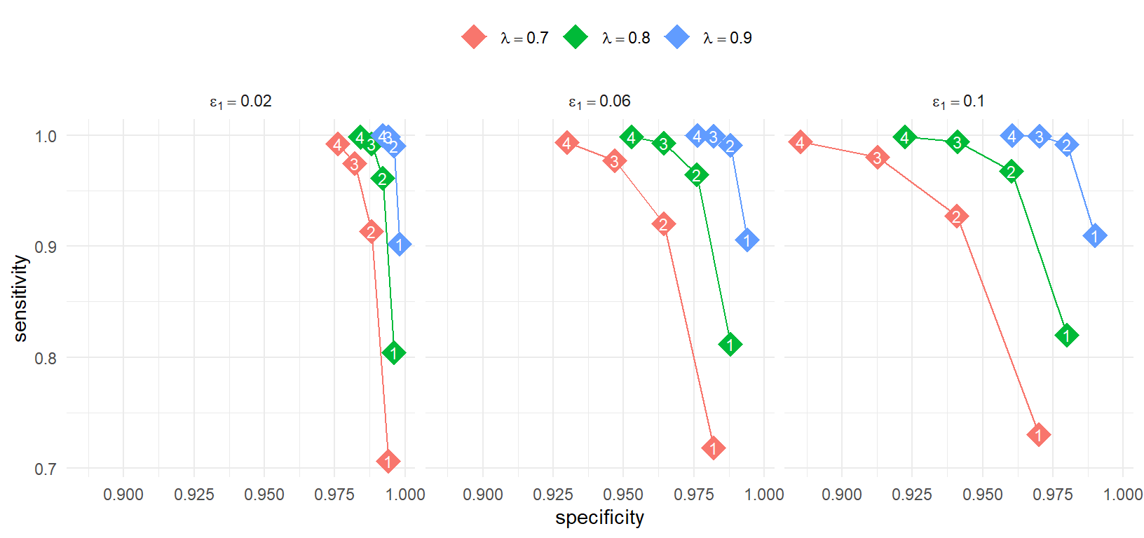
@fig-sensitivity-specificity games this out for a couple of different scenarios.
Each panel corresponds to a different probability of guessing that a record is probably relevant, from 2% (on the left) to 10% (on the right).
Within the panel, each curve shows how sensitivity (vertical axis) and specificity (horizontal axis) change as a function of the number of reviewers.
The different colors correspond to different discernment rates of 0.7 (red), 0.8 (green), or 0.9 (blue).
```{r}
#| label: fig-sensitivity-specificity
#| fig-cap: Sensitivity and specificity curves under the basic agreement model, for various values of $\epsilon_1$ and $\lambda$
#| fig-width: 8.5
#| fig-height: 4
library(tidyverse)

N <- 4000

sens_spec <-
  expand_grid(
    A = c(1,2,3,4),
    lambda = c(0.7,0.8,0.9),
    epsilon1 = c(0.02, 0.06, 0.10)
  ) %>%
  mutate(
    epsilon1_lab = paste("epsilon[1] ==", epsilon1),
    lambda_lab = paste("lambda ==", lambda),
    sensitivity = 1 - (1 - lambda)^A * (1 - epsilon1)^A,
    specificity = (lambda + (1 - lambda) * (1 - epsilon1))^A,
    relevant_missed = N * epsilon1 * (1 - sensitivity),
    irrelevant_included = N * (1 - epsilon1) * (1 - specificity)
  )

ggplot(sens_spec) +
  aes(specificity, sensitivity, color = lambda_lab, label = A) +
  geom_point(size = 6, shape = 18) +
  geom_line() +
  geom_text(color = "white", size = 3) +
  facet_wrap(
    ~ epsilon1_lab,
    labeller = label_parsed
  ) +
  scale_color_discrete(labels = scales::parse_format()) +
  theme_minimal() +
  labs(color = "") +
  theme(legend.position = "top")
```
I see a couple of interesting lessons in this plot.
First, the discernment rate (which, remember, is a function of $\kappa$) matters quite a bit for sensitivity.
With two reviewers, discernment of 0.7 leads to sensitivity of less than 95% across all three yield rates, which many reviewers would be pretty unhappy about.
Second, the gain in sensitivity from adding a third or fourth reviewer depends strongly on $\lambda$: if you have two very discerning reviewers, adding a third has very limited benefit, but doing so could meaningfully improve sensitivity if they are less discerning.
Third, the guessing distribution has much more influence on specificity than on sensitivity.
In case your brain is like mine and can't keep sensitivity and specificity straight, here's an even more tangible way to think about these scenarios.
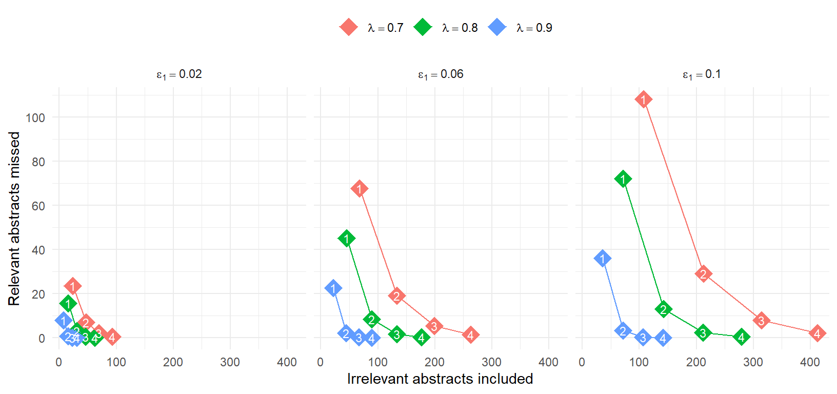
Say that we have $N = `{r} N`$ records to screen, of which $`{r} N` \tau_1$ are potentially relevant and $`{r} N` (1 - \tau_1)$ are irrelevant. We can multiply these counts by the complements of sensitivity and specificity to find, respectively, the number of relevant records that are _missed_ and the number of irrelevant records that are included.
To carry out these calculations, we'll need to add an additional assumption about the true yield.
For sake of simplicity, I'll assume that reviewers are unbiased, so $\tau_1 = \epsilon_1$.
@fig-missed-included shows these projections, following the same layout as @fig-sensitivity-specificity but with the number of relevant records missed on the vertical axis and the number of irrelevant records included on the horizontal axis.
The general lessons are the same, although the assumed yield now has a more meaningful influence on both of these quantities.
```{r}
#| label: fig-missed-included
#| fig-cap: Projected number of relevant records missed and irrelevant records included under the basic agreement model, for various values of $\epsilon_1$ and $\lambda$
#| fig-width: 8.5
#| fig-height: 4
ggplot(sens_spec) +
  aes(irrelevant_included, relevant_missed, color = lambda_lab, label = A) +
  geom_point(size = 6, shape = 18) +
  geom_line() +
  geom_text(color = "white", size = 3) +
  facet_wrap(
    ~ epsilon1_lab,
    labeller = label_parsed
  ) +
  scale_color_discrete(labels = scales::parse_format()) +
  scale_y_continuous(breaks = seq(0,100,20)) +
  theme_minimal() +
  labs(
    x = "Irrelevant abstracts included",
    y = "Relevant abstracts missed",
    color = ""
  ) +
  theme(legend.position = "top")
```
These projected quantities seem very natural to reason about. For instance, suppose we have a yield of $\tau_1 = .06$, so a total of 240 truly relevant records.
Two relatively undiscerning reviewers $(\lambda = 0.7)$ will miss about 20 records that should be included---yikes!---and will include over 130 irrelevant abstracts that will need to be screened out at a later stage.
Adding a third reviewer would reduce the number of missed records to just 5, at a cost of about 70 more irrelevant abstracts included (above and beyond the cost of the third reviewer's effort).
In contrast, two very discerning reviewers $(\lambda = 0.9)$ will miss only 2 records that should be included and will include only 45 irrelevant abstracts.
## More about agreement models
The assumptions behind the basic agreement model are non-trivial and so will need to be scrutinized when applying this sort reasoning to systematic review screening processes.
@Albert2004cautionary looked at a variety of latent class models for multi-rater classification data.
Although they did not examine the basic agreement model specifically, they demonstrate that sensitivity and specificity projections based on various latent class models can be quite discrepant from one another, even though the models may have similar fit for datasets of typical dimension.
It will be important to consider whether similar issues crop up in applying agreement models to systematic review data.
In practice, it would also be useful to consider more flexible models that work under weaker assumptions.
For instance, @Klauer1996structural noted that reviewer discernment probabilities can be allowed to _differ_ if you have at least $A \geq 3$ ratings per record.
Approaches that are very similar to the basic agreement model have appeared in a variety of different, rather disconnected literatures:
- The basic agreement model with heterogeneous discernment probabilities is a special case of the observer error models proposed by @Dawid1979maximum [see also @Passonneau2014benefits].
- @GuggenmoosHolzmann1998kappalike used a model that is essentially equivalent to the basic agreement model sketched above to interpret $\kappa$ and other agreement indices for medical diagnostic studies [see also @GuggenmoosHolzmann1996meaning].
Like @Klauer1996structural, they noted that other agreement indices besides Cohen's $\kappa$ can be derived from different assumptions about the guessing distribution.
They also give examples involving both inter-rater and _intra_-rater agreement studies (in the latter, the same person rates the same item multiple times).
- @Kiyomi2003multivariate extended the basic agreement model to multivariate categorical ratings, where each variate is categorized by multiple raters.
- @Hovy2013learning applied a version of the basic agreement model with heterogeneous discernment probabilities to analyze crowd-sourced classification decisions.
The typical setting they considered is one with a large number of reviewers (in total) and a larger number of ratings per item, although not every reviewer necessarily sees every item.
Their model also allowed the guessing distribution to differ from the consensus class distribution and allowed different reviewers to follow different guessing distributions, motivated by the notion that some reviewers are "spammers" who have very low discernment and have different button-mashing tendencies.
- @Paun2018comparing demonstrated how to fit a flexible version of the basic agreement model [as well as the @Dawid1979maximum model and several other latent class models for multi-rater classification data] using the Stan probabilistic programming language, with data drawn from natural language processing applications.
- @Moss2023measuring provided a comprehensive study of the interpretation and estimation of different agreement indices (not just Cohen's $\kappa$ but also Fleiss's version and others) defined under the basic agreement model.
- @Han2026hierarchical proposed a generalization of the (already quite general!) @Dawid1979maximum model that allows heterogeneity in the _record_ characteristics, using formulations that look like full-on item response models.
Considering that the basic agreement model has cropped up in so many different contexts (and across multiple, apparently disconnected methodological literatures), it seems worth investigating further whether it could be useful for interpreting systematic review screening processes.
The connection to Cohen's $\kappa$ is helpful on a pragmatic level because $\kappa_{ab}$ is one of the few scraps of information commonly reported about screening processes.
Ultimately though, what seems more intriguing to me is the possibility of developing useful _models_ for reasoning about how to do this stage of a systematic review more effectively and efficiently.