Code
sigma_i <- 2 / sqrt(rpois(10000, lambda = 30))For one of her dissertation studies, my advisee Paulina Grekov is looking at factors that influence the performance of publication bias adjustment methods in meta-analysis (e.g., methods like Trim-and-Fill, PET-PEESE, and the three-parameter selection model). Of course, there is already a large literature about these methods, including many simulation studies that have looked at adjustment methods under a range of different conditions (e.g., Bramley et al., 2021; Carter et al., 2019; McShane et al., 2016; Stanley & Doucouliagos, 2014; van Aert & van Assen, 2026, to name but a few). Past simulations have looked at a variety of bias-detection and bias-adjustment methods under a wide variety of different data-generating processes, varying in the metric of the simulated effect size estimates, the distribution of primary study sample sizes, the form and strength of selective reporting, and other factors. Hong & Reed (2021) reviewed many of these past studies, demonstrating that differences in the conditions examined (what they call the simulation environment) lead to discrepant findings about the performance of some methods. How well the bias-adjustment methods work (and which method or methods should be used in practice) seems to depend on how the data were generated, such as the degree of heterogeneity, how large the simulated studies are, and how severe the selection bias is.
Something that makes it challenging to compare findings across these past studies is that they use different procedures for simulating meta-analytic datasets. Many past studies simulated datasets based on some more-or-less simple form of step-function selection model, such as the so-called three-parameter selection model (3PSM) that has a single step at \(\alpha = .025\). But there are different ways to actually program this, and it’s a little tricky to line them up. In this post, I’ll look at two such methods: one used by McShane et al. (2016) and one by Stanley & Doucouliagos (2014).
The 3PSM posits that effect size estimates are observed based on a two-step process. First, estimates are generated (but potentially not observed) based on a random effects model, in which \[ \left(T_i^* | \sigma_i^*\right) \sim N\left(\mu, \ \tau^2 + {\sigma_i^*}^2\right), \tag{1}\] where I use the asterisks on \(T_i^*\) and \(\sigma_i^*\) to indicate that the estimates are generated but not necessarily observed. Second, the effects are censored according to whether their one-sided p-values are above or below \(\alpha_1 = .025\). Let me denote the one-sided p-value as \(p_i^* = 1 - \Phi^{-1}(T_i^* / \sigma_i^*)\), let \(A_i^* = I(p_i^* < \alpha_1)\) be an indicator for whether effect size estimate \(i\) is affirmative (positive and statistically significant), and let \(O_i\) be a binary indicator for whether \(\left(T_i^*, \sigma_i^*\right)\) is observed. The 3PSM posits that \[ \Pr(O_i = 1 | T_i^*, \sigma_i^*) = A_i^* + \lambda_1 (1 - A_i^*), \tag{2}\] so if \(p_i^* \geq \alpha_1\), then \(\left(T_i^*, \sigma_i^*\right)\) is observed with probability \(\lambda_1\) and censored with probability \(1 - \lambda_1\).
As described in my earlier post, these assumptions lead to a distributional model for the observed effect size estimates that is piece-wise normal. Letting \(\eta_i = \sqrt{\tau^2 + \sigma_i^2}\) and \(c_{1i} = \left[\sigma_i \Phi^{-1}(1 - \alpha_1) - \mu\right] / \eta_i\), the density of an observed effect size estimate is given by \[ \Pr(T_i = t | \sigma_i) = \frac{a_i + \lambda_1 (1 - a_i)}{1 - (1 - \lambda_1) \Phi(c_{1i})} \times \frac{1}{\eta_i}\phi\left(\frac{t - \mu}{\eta_i}\right), \tag{3}\] where \(a_i = I\left[(1 - \Phi^{-1}(t / \sigma_i) < \alpha_1\right]\) is an indicator for whether an effect of size \(t\) is affirmative.
McShane et al. (2016) simulated from the 3PSM using a stochastic selection process that aligns very closely with the formulation of the model. Their approach is as follows:
They repeat this until they end up with a dataset that includes a total of \(K\) observed effect size estimates.
To compare their approach to other approaches, I will need the marginal probability of observing an affirmative effect and the unconditional expectation of \(T_i\). Now, conditional on a generated \(\sigma_i^*\), \[ \Pr(A_i^* = 1, O_i = 1 | \sigma_i^*) = \Pr(A_i^* = 1 | \sigma_i^*) = 1 - \Phi(c_{1i}). \tag{4}\] Likewise, conditional on \(\sigma_i\) (but not on \(T_i\)), \[ \Pr(O_i = 1 | \sigma_i^*) = 1 - (1 - \lambda_1) \Phi(c_{1i}). \tag{5}\] Letting \(\mathbb{E}\) be the expectation with respect to the generating distribution of \(\sigma_i^*\), the corresponding marginal probabilities are \(\Pr(A_i^* = 1, O_i = 1) = 1 - \mathbb{E}\left[\Phi(c_{1i})\right]\) and \(\Pr(O_i = 1) = 1 - (1 - \lambda_1) \mathbb{E}\left[\Phi(c_{1i})\right]\). Thus, \[ \Pr(A_i^* = 1 | O_i = 1) = \frac{\Pr(A_i^* = 1, O_i = 1)}{\Pr(O_i = 1)} = \frac{1 - \mathbb{E}\left[\Phi(c_{1i})\right]}{1 - (1 - \lambda_1) \mathbb{E}\left[\Phi(c_{1i})\right]}. \tag{6}\]
Under the 3PSM, the conditional expected value of the observed effect size estimate is \[ \mathbb{E}(T_i | \sigma_i) = \mu + \eta_i \times \frac{(1 - \lambda_1) \phi(c_{1i})}{1 - (1 - \lambda_1)\Phi(c_{1i})}. \tag{7}\] It’s perhaps a bit weird to worry about the unconditional expectation, considering that meta-analysts will typically focus on weighted averages of the effect size estimates, as in a random effects model. In practice, the weights will depend on estimation of the between-study heterogeneity \(\tau\), but we can gloss over this by considering random effects weights based on the true value of \(\tau\). Because this quantity won’t actually ever be known in real life, I’ll call this the oracle-weighted expectation. First, let me define \[ \begin{aligned} \omega_S &= \mathbb{E}(\eta_i^{-2} | O_i = 1) \\ &= \frac{\mathbb{E}\left[\eta_i^{-2} \Pr(O_i = 1 | \sigma_i^*) \right]}{\mathbb{E}\left[\Pr(O_i = 1 | \sigma_i^*) \right]} \\ &= \frac{\mathbb{E}\left[\eta_i^{-2} \left(1 - (1 - \lambda_1) \Phi(c_{1i})\right) \right]}{1 - (1 - \lambda_1) \mathbb{E}\left[\Phi(c_{1i})\right]} \end{aligned} \tag{8}\] The marginal oracle-weighted expectation of \(T_i\) is then \[ \begin{aligned} \frac{ 1}{\omega_S} \mathbb{E}\left(\left. \eta_i^{-2} T_i \right| O_i = 1\right) &= \frac{\mathbb{E}\left[\eta_i^{-2} \mathbb{E}\left(T_i | O_i = 1, \sigma_i^*\right) \Pr(O_i = 1 | \sigma_i^*) \right]}{\omega_S \times \mathbb{E}\left[\Pr(O_i = 1 | \sigma_i^*) \right]} \\ &= \frac{\mathbb{E}\left[\eta_i^{-2} \left(\mu + \eta_i \frac{(1 - \lambda_1) \phi(c_{1i})}{1 - (1 - \lambda_1)\Phi(c_{1i})}\right) \left(1 - (1 - \lambda_1) \Phi(c_{1i})\right) \right]}{\omega_S \times \mathbb{E}\left[\Pr(O_i = 1 | \sigma_i^*) \right]} \\ &= \mu + \left(1 - \lambda_1 \right) \times \frac{\mathbb{E}\left[\eta_i^{-1} \phi(c_{1i})\right]}{\mathbb{E}\left[\eta_i^{-2}\right] - (1 - \lambda_1) \mathbb{E}\left[\eta_i^{-2}\Phi(c_{1i})\right]}. \end{aligned} \tag{9}\] I’ll circle back to this expression in a bit.
Stanley & Doucouliagos (2014) and Stanley (2017) reported simulations based on a subtly different appoach to implementing the selective reporting process. Rather than treating the selection process as stochastic, given the p-value of the generated effect size estimate, they conceptualized the process as a mixture of two types of studies (or two types of researchers). One type of researcher, comprising \(\pi_1\) of the population of observed researchers, reports all results regardless of whether they are affirmative. The other type of researcher, comprising the remaining \(1 - \pi_1\) of the observed population, only reports results that are affirmative (positive and statistically significant). Every meta-analytic dataset consists of \(k \times \pi_1\) effect size estimates generated by the first type of researcher and \(k \times (1 - \pi_1)\) effect size estimates generated by the second type.1 Both types of researchers draw primary study sample sizes from the same distribution (i.e., researcher type is independent of \(\sigma_i^*\)).
In the Stanley & Doucouliagos (2014) simulation approach, the observed effect size estimates follow a mixture distribution in which \[ \begin{aligned} \Pr(T_i = t | \sigma_i) &= \pi_1 \times \frac{1}{\eta_i}\phi\left(\frac{t - \mu}{\eta_i}\right) + (1 - \pi_1) \times \frac{a_i \phi\left(\frac{t - \mu}{\eta_i}\right)}{\eta_i\left[1 - \Phi(c_{1i}) \right]} \\ &= \left[\pi_1+ (1 - \pi_1) \times \frac{a_i}{\left[1 - \Phi(c_{1i}) \right]} \right] \times \frac{1}{\eta_i}\phi\left(\frac{t - \mu}{\eta_i}\right), \end{aligned} \tag{10}\] with conditional expectation \[ \mathbb{E}(T_i | \sigma_i) = \mu + \eta_i \times \frac{(1 - \pi_1) \phi(c_{1i})}{1 - \Phi(c_{1i})}. \tag{11}\] Let \(G_i\) be a latent indicator for the first (unbiased) type of study. Under this approach, \[ \begin{aligned} \Pr(A_i^* = 1 | O_i = 1) &= \pi_1 \times \Pr(A_i^* = 1 | O_i = 1, G_i = 1) \\ & \qquad \qquad + (1 - \pi_1) \times \Pr(A_i^* = 1 | O_i = 1, G_i = 0) \\ &= \pi_1 \times \Pr(A_i^* = 1 | G_i = 1) + (1 - \pi_1) \times 1 \\ &= \pi_1 \left[1 - \mathbb{E}\left[\Phi(c_{1i})\right]\right] + (1 - \pi_1) \\ &= 1 - \pi_1 \mathbb{E}\left[\Phi(c_{1i})\right]. \end{aligned} \tag{12}\] Under the Stanley & Doucouliagos (2014) approach, the expected inverse variance weight is \[ \begin{aligned} \omega_M &= \mathbb{E}(\eta_i^{-2} | O_i = 1) \\ &= \pi_1 \mathbb{E}(\eta_i^{-2} | O_i = 1, G = 1) + (1 - \pi_1) \mathbb{E}(\eta_i^{-2} | O_i = 1, G = 0) \\ &= \pi_1 \mathbb{E}\left(\eta_i^{-2}\right) + (1 - \pi_1) \frac{\mathbb{E}\left[\eta_i^{-2}(1 - \Phi(c_{1i})) \right]}{\mathbb{E}\left[1 - \Phi(c_{1i}) \right]} \\ \end{aligned} \tag{13}\] and the unconditional, oracle-weighted expectation of an observed effect size is \[ \begin{aligned} \frac{1}{\omega_M}\mathbb{E} \left[ \eta_i^{-2} T_i | O_i = 1 \right] &= \frac{1}{\omega_M} \left[ \pi_1 \mathbb{E}(\eta_i^{-2} T_i | O_i = 1, G = 1) + (1 - \pi_1) \mathbb{E}(\eta_i^{-2} | O_i = 1, G = 0)\right] \\ &= \frac{1}{\omega_M} \left[\pi_1 \mu \mathbb{E}(\eta_i^{-2}) + (1 - \pi_1) \frac{\mathbb{E}\left[\eta_i^{-2} \mathbb{E}(T_i | O_i = 1, \sigma_i^*, G = 0) \Pr(O_i = 1 | \sigma_i^*, G = 0) \right]}{\mathbb{E}\left[\Pr(O_i = 1 | \sigma_i^*, G = 0) \right]}\right] \\ &= \frac{1}{\omega_M} \left[\pi_1 \mu \mathbb{E}(\eta_i^{-2}) + (1 - \pi_1) \frac{\mathbb{E}\left[\eta_i^{-2} \left(\mu + \eta_i \frac{\phi(c_{1i})}{1 - \Phi(c_{1i})} \right) \left( 1 - \Phi(c_{1i}) \right) \right]}{\mathbb{E}\left[1 - \Phi(c_{1i}) \right]}\right] \\ &= \mu + \frac{1 - \pi_1}{\omega_M} \frac{\mathbb{E}\left[\eta_i^{-1}\phi(c_{1i})\right]}{\mathbb{E}\left[1 - \Phi(c_{1i}) \right]} \\ &= \mu + \frac{(1 - \pi_1)\mathbb{E}\left[\eta_i^{-1}\phi(c_{1i})\right]}{\pi_1 \mathbb{E}\left[\eta_i^{-2}\right]\mathbb{E}\left[1 - \Phi(c_{1i}) \right] + (1 - \pi_1) \mathbb{E}\left[\eta_i^{-2}\left(1 - \Phi(c_{1i})\right) \right]}. \end{aligned} \tag{14}\]
The question is then how the mixing proportion \(\pi_1\) relates to the selection parameter \(\lambda_1\). If we wanted to directly equate the distributions for a given standard error \(\sigma_i\), we could set the mixing proportion to \[ \pi_{1i} = \frac{\lambda_1}{1 - (1 - \lambda_1)\Phi(c_{1i})}. \tag{15}\] The difficulty here is that the mixing proportion is a function of the standard error for effect size \(i\), so studies with different standard errors would need to have different mixing proportions. That’s not how Stanley & Doucouliagos (2014) implement their data-generating process, so it doesn’t really work as a way to translate between the selection parameter and the mixing proportion. However, we could try to equate the expected proportion of affirmative effects observed under both approaches. Setting Equation 6 equal to Equation 12 leads to \[ \pi_1 = \frac{\lambda_1}{1 - (1 - \lambda_1) \mathbb{E}\left[\Phi(c_{1i})\right]}, \tag{16}\] which amounts to just substituting the marginal probability of a non-significant result in place of the corresponding probability conditional on \(\sigma_i\). Note that the translation from \(\lambda_1\) to \(\pi\) will generally depend on all the parameters of the model as well as on the distribution of the observed \(\sigma_i\)’s.
Computing \(\pi_1\) will require some way of approximating the expectations in Equation 16. If \(\sigma_i\) only takes on a finite set of distinct values, the expectation could be computed directly. Otherwise, stochastic approximation could be used. For instance, suppose that \(4 / \sigma_i^2 \sim Poisson(30)\), so we can simulate a large set of \(\sigma_i\)’s by taking
sigma_i <- 2 / sqrt(rpois(10000, lambda = 30))Given values for the other model parameters, we compute the expectations by averaging over all the \(\sigma_i\)’s. Here is a function that computes \(\pi_1\) given \(\mu\), \(\tau\), \(\lambda_1\), \(\alpha_1\), and a vector of \(\sigma_i\) values:
mixing_prop <- function(
  mu, tau, lambda_1, sigma_i,
  alpha_1 = .025
) {
  eta_i <- sqrt(tau^2 + sigma_i^2)
  c_1i <- (sigma_i * qnorm(1 - alpha_1) - mu) / eta_i
  EP_1 <- mean(pnorm(c_1i))
  pi_1 <- lambda_1 / (1 - (1 - lambda_1) * EP_1)
  return(pi_1)
}

mixing_prop(mu = 0.2, tau = 0.1, lambda_1 = 0.2, sigma_i = sigma_i)
[1] 0.7428932library(tidyverse)
param_grid <-
expand_grid(
mu = seq(0.0, 0.6, 0.2),
tau = seq(0.0, 0.4, 0.1),
lambda_1 = seq(0, 1, 0.02)
) %>%
mutate(
mu_f = formatC(mu, format = "f", digits = 1) |>
fct() |>
fct_relabel(\(x) paste("mu ==", x)),
tau_f = formatC(tau, format = "f", digits = 1) |> fct(),
pi_1 = pmap_dbl(
.l = list(mu = mu, tau = tau, lambda_1 = lambda_1),
.f = mixing_prop,
sigma_i = sigma_i
)
)
ggplot(param_grid) +
aes(lambda_1, pi_1, color = tau_f) +
geom_line() +
facet_wrap(~ mu_f, labeller = "label_parsed") +
theme_minimal() +
theme(legend.position = "top") +
labs(
x = expression(lambda[1]),
y = expression(pi[1]),
color = expression(tau)
)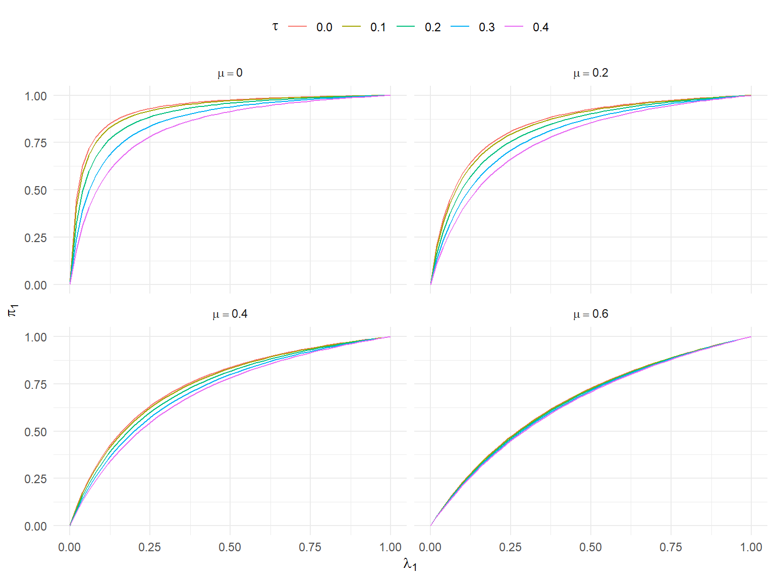
Figure 1 shows how the mixing proportion changes as a function of the selection parameter \(\lambda_1\) for several different values of the average effect size \(\mu\) and between-study heterogeneity \(\tau\), using the same set of \(\sigma_i\) values simulated above. It is a fairly complicated function. For smaller average effects, the degree of heterogeneity has relatively more influence on the shape of the function, whereas for larger average effects, the degree of heterogeneity hardly matters. And everything depends on the \(\sigma_i\) distribution; changing it would shift all of the curves depicted.
One question about this approach to equating is what it implies about the oracle-weighted expected effect sizes under each approach. I’ve provided expressions for this quantity under both approaches. Substituting Equation 16 into Equation 14 yields \[ \frac{1}{\omega_M}\mathbb{E} \left[ \eta_i^{-2} T_i | O_i = 1 \right] = \mu + \left(1 - \lambda_1\right) \frac{\mathbb{E}\left[\eta_i^{-1} \phi(c_{1i}) \right]}{\mathbb{E}\left[\eta_i^{-2} \right] + (1 - \lambda_1)\mathbb{E}\left[\eta_i^{-2}\Phi(c_{1i}) \right]} \tag{17}\] which is indeed the same as Equation 9. Thus, equating the probability of observing a significant effect also leads to equating the oracle-weighted expected effects.
Paulina’s simulation work also considers a more general version of a step-function selection model with steps at both \(\alpha_1 = .025\) and \(\alpha_2 = .500\)–a four-parameter selection model (4PSM), if you will. If we let \(M_i = I(\alpha_1 \leq p_i^* < \alpha_2)\) and \(N_i = I(\alpha_2 \leq p_i^*)\), the selection process is \[ \Pr(O_i = 1 | T_i^*, \sigma_i^*) = N_i \lambda_2 + M_i \lambda_1 + (1 - M_i - N_i). \tag{18}\] Following a data-generating process like the McShane et al. (2016) approach, the probability that an effect is observed, conditional only on \(\sigma_i^*\), is \[ \Pr(O_i = 1 | \sigma_i^*) = 1 - \Phi(c_{1i}) + \lambda_1 \left[\Phi(c_{1i}) - \Phi(c_{2i}) \right] + \lambda_2 \Phi(c_{2i}). \tag{19}\] where \(c_{1i} = \left[\sigma_i \Phi^{-1}(1 - \alpha_1) - \mu\right] / \eta_i\) (as before) and \(c_{2i} = \left[\sigma_i \Phi^{-1}(1 - \alpha_2) - \mu\right] / \eta_i\). Further, the marginal probability of observing a negative effect is \[ \Pr(N_i = 1 | O_i) = \frac{\lambda_2 \mathbb{E}\left[\Phi(c_{2i})\right]}{1 - (1 - \lambda_1) \mathbb{E}\left[\Phi(c_{1i})\right] - (\lambda_1 - \lambda_2) \mathbb{E}\left[\Phi(c_{2i})\right]}, \] the marginal probability of observing a positive but non-significant effect is \[ \Pr(M_i = 1 | O_i) = \frac{\lambda_1 \mathbb{E}\left[\Phi(c_{1i}) - \Phi(c_{2i})\right]}{1 - (1 - \lambda_1) \mathbb{E}\left[\Phi(c_{1i})\right] - (\lambda_1 - \lambda_2) \mathbb{E}\left[\Phi(c_{2i})\right]}, \] and the conditional expectation of an observed effect size estimate is \[ \mathbb{E}(T_i | \sigma_i) = \mu + \eta_i \times \frac{(1 - \lambda_1) \phi(c_{1i}) + (\lambda_1 - \lambda_2) \phi(c_{2i})}{1 - (1 - \lambda_1)\Phi(c_{1i}) - (\lambda_1 - \lambda_2) \Phi(c_{2i})}. \tag{20}\]
How would the Stanley & Doucouliagos (2014) approach work with more than a single step? One way to generalize it would be to think of the observed effect sizes as a three-component mixture, where there is a fraction of studies \(\pi_2\) where an effect size estimate is always reported regardless of sign or statistical significance, another fraction of studies \(\pi_1\) where an effect size estimate is reported only when \(p_i^* < \alpha_2\) (i.e., when the effect size estimate is larger than zero), and the remaining faction \(1 - \pi_1 - \pi_2\) where an effect size estimate is reported only when \(p_i^* < \alpha_1\). Clearly, this requires that \(\pi_1 \geq 0\), \(\pi_2 \geq 0\), and \(\pi_1 + \pi_2 \leq 1\); Under this data-generating process, \[ \begin{aligned} \Pr(N_i = 1 | O_i) &= \pi_2 \mathbb{E}\left[\Phi(c_{2i})\right], \\ \Pr(M_i = 1 | O_i) &= \mathbb{E}\left[\Phi(c_{1i}) - \Phi(c_{2i})\right] \left(\pi_2 + \frac{\pi_1}{1 - \mathbb{E}\left[\Phi(c_{2i})\right]}\right), \end{aligned} \] and the conditional expectation of an observed effect size estimate is \[ \mathbb{E}(T_i | \sigma_i) = \mu + \eta_i \times \left[\frac{\pi_1 \phi(c_{2i})}{1 - \Phi(c_{2i})} + \frac{(1 - \pi_1 - \pi_2) \phi(c_{1i})}{1 - \Phi(c_{1i})}\right]. \tag{21}\] To compare this data-generating approach to the McShane et al. (2016) approach, we need to be able to translate from \(\left(\lambda_1, \lambda_2\right)\) to \(\left(\pi_1, \pi_2\right)\), at least for selection parameters where \(0 \leq \lambda_2 \leq \lambda_1 \leq 1\).
Just as with the simpler single-step model, one way to calibrate the model parameters is to equate the marginal proportions of effects observed within each range of p-values. Doing so leads to \[ \begin{aligned} \pi_1 &= \frac{\left(\lambda_1 - \lambda_2\right)\left(1 - \mathbb{E}(\Phi(c_{2i}))\right)}{1 - (1 - \lambda_1) \mathbb{E}\left[\Phi(c_{1i})\right] - (\lambda_1 - \lambda_2) \mathbb{E}\left[\Phi(c_{2i})\right]} \\ \pi_2 &= \frac{\lambda_2}{1 - (1 - \lambda_1) \mathbb{E}\left[\Phi(c_{1i})\right] - (\lambda_1 - \lambda_2) \mathbb{E}\left[\Phi(c_{2i})\right]}. \end{aligned} \tag{22}\] When \(\lambda_2 = \lambda_1\), \(\pi_1 = 0\) and \(\pi_2\) then maps directly to \(\lambda_1\) in the same way as under the simpler, single-step model, as given in Equation 16. When \(\lambda_1 = 1\), then \(\pi_1 + \pi_2 = 1\) and \(\pi_2 = \lambda_2 / \left[1 - (1 - \lambda_2)\mathbb{E}\left[\Phi(c_{2i})\right] \right]\), which is analogous to Equation 16 but with \(\lambda_2\) in place of \(\lambda_1\) and \(c_{2i}\) in place of \(c_{1i}\). Finally, as one would expect, \(\lambda_2 = 0\) implies that \(\pi_2 = 0\) and \(\lambda_1 = \lambda_2 = 0\) implies that \(\pi_1 = \pi_2 = 0\).
Here is a function that computes \(\left(\pi_1,\pi_2\right)\) given \(\mu\), \(\tau\), \(\lambda_1\), \(\lambda_2\), \(\alpha_1\), \(\alpha_2\), and a vector of \(\sigma_i\) values:
mixing_prop2 <- function(
  mu, tau, lambda_1, lambda_2, sigma_i,
  alpha_1 = .025, alpha_2 = .500
) {

  eta_i <- sqrt(tau^2 + sigma_i^2)
  c_1i <- (sigma_i * qnorm(1 - alpha_1) - mu) / eta_i
  c_2i <- (sigma_i * qnorm(1 - alpha_2) - mu) / eta_i
  EP_1 <- mean(pnorm(c_1i))
  EP_2 <- mean(pnorm(c_2i))
  denom <- 1 - (1 - lambda_1) * EP_1 - (lambda_1 - lambda_2) * EP_2
  pi_1 <- (lambda_1 - lambda_2) * (1 - EP_2) / denom
  pi_2 <- lambda_2 / denom
  return(data.frame(pi_1 = pi_1, pi_2 = pi_2))
}

mixing_prop2(mu = 0.2, tau = 0.1, lambda_1 = 0.4, lambda_2 = 0.1, sigma_i = sigma_i)
pi_1 pi_2
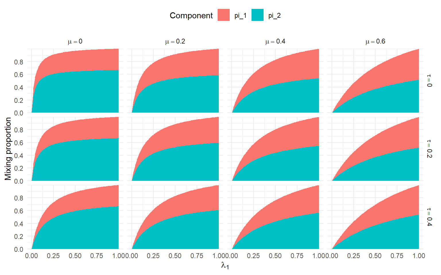
1 0.580343 0.2762478Figure 2 shows how the mixture proportions change as \(\lambda_1\) varies when the probability of observing a negative effect is pegged at \(\lambda_2 = 0.5 \lambda_1\). Just as with the simpler single-step case, the mixture probabilities are a complicated function of the selection parameters, the \(\mu\) and \(\tau\) parameters that control the distribution of effect sizes prior to selection, and the distribution of \(\sigma_i^*\) values used to generate studies. The curves are strongly affected by \(\mu\), and tend to be more affected by \(\tau\) when \(\mu\) is small and less sensitive to \(\tau\) when \(\mu\) is larger.
library(tidyverse)
param_grid_4PSM <-
  expand_grid(
    mu = seq(0.0, 0.6, 0.2),
    tau = seq(0.0, 0.4, 0.2),
    lambda_1 = seq(0, 1, 0.02)
  ) %>%
  mutate(
    lambda_2 = 0.5 * lambda_1,
    mu_f = formatC(mu, format = "f", digits = 1) |>
      fct() |>
      fct_relabel(\(x) paste("mu ==", x)),
    tau_f = formatC(tau, format = "f", digits = 1) |>
      fct() |>
      fct_relabel(\(x) paste("tau ==", x)),
    pmap_dfr(
      .l = list(mu = mu, tau = tau, lambda_1 = lambda_1, lambda_2 = lambda_2),
      .f = mixing_prop2,
      sigma_i = sigma_i
    )
  ) %>%
  pivot_longer(
    starts_with("pi_"),
    names_to = "component",
    values_to = "prop"
  )

ggplot(param_grid_4PSM) +
  aes(lambda_1, prop, fill = component) +
  geom_area() +
  facet_grid(tau_f ~ mu_f, labeller = "label_parsed") +
  scale_y_continuous(
    limits = c(0,1),
    expand = expansion(0,0),
    breaks = seq(0,0.8,0.2)
  ) +
  theme_minimal() +
  theme(legend.position = "top") +
  labs(
    x = expression(lambda[1]),
    y = "Mixing proportion",
    fill = "Component"
  )
Note that this approach to generating data involves controlling the mixing proportion of observed researchers, thereby ensuring that at least \(k \times (1 - \pi_1)\) observed effects will be affirmative.↩︎