Pusto’s package downloads

Back in 2019, I posted an analysis of the R packages that I have developed, looking at how frequently they have been downloaded, comparing them to other topically related packages, and examining time trends in download frequency. I was coming up for tenure review at that point and so wanted to provide a little bit of data about the software tools that I’d worked on, even though (at my institution, at least) these weren’t really understood as academic contributions like journal articles or books or whatnot.

These days, I’m (happily) tenured at a different university, still developing some R packages, but my work has become much more collaborative. Of the four R packages that I looked at in 2019, two were solo projects (clubSandwich and ARPobservation) and two were my design, with some contributions from students (SingleCaseES and scdhlm). I’ve since been involved with five additional R packages (lmeInfo, metaselection, POMADE, simhelpers, and wildmeta)—all developed in collaboration with students—and my packages related to single-case effect sizes have seen major contributions from student collaborators. In short, the packages are no longer mine, but rather represent tools to which I’ve contributed. I’m no less proud of the products, though.

Since it has been over seven years since my previous post on package downloads, I felt like it was time for an updated look. I’ll follow more or less the same methodology as before, using statistics from METACRAN. The site makes available data on daily downloads from the RStudio mirror of CRAN, which is just one of many mirrors around the world. Although the data do not represent complete tallies of all package downloads, as far as I know, it is still the best available source of this sort of data.

Comparison packages

The nine packages that I’ve developed or contributed to do a variety of things, but the dominant theme is meta-analysis and effect size calculation. Here’s how I’m thinking about packages to use as points of comparison:

• POMADE does power calculations for meta-analysis with dependent effect sizes. Comparison package: PowerUpR, a general power analysis package with included Shiny app.
• wildmeta implements bootstrap tests for meta-analytic models. Comparison packages: bayesmeta and metaforest, which both do specialized meta-analysis stuff.
• metaselection implements several estimators for meta-analytic selection models, with inference methods that handle dependent effect size estimates. This package is brand new so I will exclude it from further analysis.
• scdhlm and SingleCaseES do effect size calculations for use in meta-analysis of single-case designs. Comparison package: compute.es does effect size calculations for a variety of generic effect size measures.
• ARPobservation provides tools for simulating behavioral observation data based on an alternating renewal process model. Comparison package: Countr provides estimation routines for renewal process models.

Some of my other packages have a broader statistical scope:

• clubSandwich provides cluster-robust variance estimators for a variety of different models (including meta-regression, hierarchical linear models, panel data models, GEE models, instrumental variables models, etc.). The obvious comparison would be sandwich, which implements a broader class of sandwich estimators for a range of different models, but without some of the small-sample corrections provided by clubSandwich. Other relevant points of comparison are packages that implement some form of cluster-robust standard errors for a certain class of models, such as plm and fixest for fixed effect models and robumeta for meta-regression models.
• lmeInfo provides analytic derivatives for hierarchical linear models estimated using nlme::lme(). Comparison package: merDeriv provides similar functionality for lme4::lmer() models; nlme, which my package enhances.
• simhelpers provides helper functions for running Monte Carlo simulations. Other packages that provide tools for Monte Carlo simulations include SimDesign, SimEngine, simFrame, simstudy, simulator, simpr, simTool, and MonteCarlo.

library(tidyverse)
library(lubridate)
library(cranlogs)
library(kableExtra)
library(ggrepel)

to_date <- as_date("2026-08-31")
file_name <- paste0("CRAN package downloads ", to_date, ".rds")
long_file_name <- paste0("CRAN package download history ", to_date, ".rds")
from_date <- as.character(as_date(to_date - duration(1, "year")))

pkg_downloads <-
  available.packages() %>%
  as_tibble() %>%
  select(Package, Version) %>%
  mutate(grp = 1 + trunc((row_number() - 1) / 100)) %>%
  nest(data = c(Package, Version)) %>%
  mutate(downloads = map(.$data, ~ cran_downloads(packages = .$Package, from = from_date))) %>%
  select(-data) %>%
  unnest(cols = downloads)

saveRDS(pkg_downloads, file = file_name)

pkg_downloads <- readRDS(file_name)

downloaded_last_yr <- 
  pkg_downloads %>%
  filter(
    date <= to_date - duration(6, "months"),
  ) %>%
  group_by(package) %>%
  summarise(
    count = sum(count)
  ) %>%
  filter(count > 0) %>%
  select(package)

downloads_past_twelve <-
  pkg_downloads %>%
  filter(date > to_date - duration(12, "months")) %>%
  semi_join(downloaded_last_yr, by = "package") %>%
  group_by(package) %>%
  summarise(
    count = sum(count) / 12
  ) %>%
  mutate(
    pct_less = 100 * cume_dist(count),
    package = fct_rev(fct_infreq(package, w = count))
  )

Downloads over the past year

I used daily download counts from the RStudio CRAN mirror from 2025-08-30 through 2026-08-31. I limited the sample to packages that had been downloaded at least once between 2025-08-30 18:00:00 and 2026-03-01. This yielded 22614 packages. For each of these packages, I then calculated the average monthly download rate over the past twelve months, along with where that rate falls as a percentile of all packages in the sample.

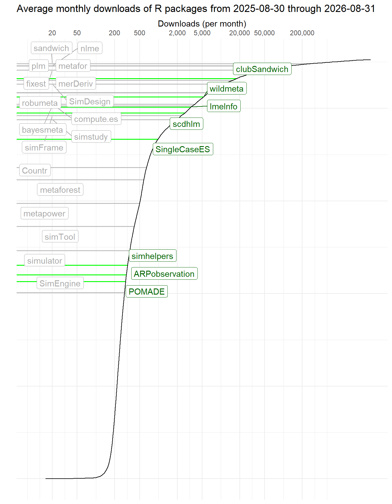
Here are the average monthly download rates for each of my packages (highlighted in blue), along with the full set of comparison packages:

comp_pkg_dat <- tribble(
  ~ Pusto_pkg, ~ Comp_pkg,
  "ARPobservation", "Countr",
  "scdhlm", "compute.es",
  "SingleCaseES", NA_character_,
  "lmeInfo", "merDeriv",
  "lmeInfo", "nlme",
  "clubSandwich", "sandwich",
  "clubSandwich", "robumeta",
  "clubSandwich", "plm",
  "clubSandwich", "fixest",
  "clubSandwich", "metafor",
  "wildmeta", "bayesmeta",
  "wildmeta", "metaforest",
  "simhelpers", "SimDesign",
  "simhelpers", "SimEngine",
  "simhelpers", "simFrame",
  "simhelpers", "simstudy",
  "simhelpers", "simulator",
  "simhelpers", "simTool",
  "POMADE", "metapower"
)

pkg_groups <- 
  comp_pkg_dat %>%
  mutate(
    group = case_match(Pusto_pkg, "SingleCaseES" ~ "scdhlm/SingleCaseES", "scdhlm" ~ "scdhlm/SingleCaseES", .default = Pusto_pkg)
  ) %>%
  pivot_longer(ends_with("_pkg"), names_to = "type", values_to = "package") %>%
  mutate(
    type = case_match(type, "Pusto_pkg" ~ "Pusto", "Comp_pkg" ~ "Comparison")
  ) %>%
  filter(!is.na(package)) %>%
  group_by(group, type, package) %>%
  summarize(.groups = "drop") %>%
  mutate(
    package = factor(package, levels = levels(downloads_past_twelve$package))
  )

Pusto_pkgs <- unique(comp_pkg_dat$Pusto_pkg)
comp_pkgs <- unique(comp_pkg_dat$Comp_pkg)
comp_pkgs <- comp_pkgs[!is.na(comp_pkgs)]

focal_package_downloads <- 
  pkg_groups %>%
  left_join(downloads_past_twelve) %>%
  arrange(desc(pct_less))
          
focal_package_downloads %>%
  select(package, count, pct_less) %>%
  rename(`Average monthly downloads` = count, `Percentage of packages with smaller download rate` = pct_less) %>%
  kable(
    table.attr = 'data-quarto-disable-processing="true"',
    digits = c(0,0,1),
    format = "html"
  ) %>%
  kable_styling(full_width = FALSE, bootstrap_options = c("responsive","hover"), fixed_thead = TRUE) %>%
  column_spec(2:3, width = "12em") %>%
  row_spec(which(focal_package_downloads$type == "Pusto"), background = "lightblue")

package	Average monthly downloads	Percentage of packages with smaller download rate
sandwich	273314	99.1
nlme	123461	98.6
metafor	52550	97.6
plm	51631	97.6
fixest	51523	97.6
clubSandwich	18200	95.6
merDeriv	15577	95.1
SimDesign	11598	94.2
robumeta	6424	92.2
wildmeta	5271	91.2
compute.es	3860	89.4
bayesmeta	3511	89.0
lmeInfo	3333	88.8
scdhlm	2668	87.3
simFrame	2329	86.7
simstudy	1984	85.8
SingleCaseES	982	81.0
Countr	646	74.3
metaforest	585	71.4
metapower	502	65.8
simTool	411	60.2
simulator	350	54.5
simhelpers	322	51.0
ARPobservation	307	48.7
POMADE	299	47.1
SimEngine	287	44.4

title_str <- paste("Average monthly downloads of R packages from", as_date(as_date(from_date)),"through",to_date)

downloads_graph <- 
  downloads_past_twelve %>%
  arrange(package) %>%
  left_join(pkg_groups, by = "package") %>%
  mutate(
    type = recode(type, .missing = "none"),
    pkg_num = as.numeric(package)
  )

focal_downloads_graph <- 
  downloads_graph %>%
  filter(!is.na(group))

p <- 
  ggplot(focal_downloads_graph) +
  aes(x = pkg_num, y = count) + 
  geom_col(aes(color = type, group = package), linewidth = 0.7) + 
  geom_line(data = downloads_graph, color = "black") + 
  scale_color_manual(values = c(Pusto = "green", Comparison = "grey")) +
  scale_y_log10(
    breaks = c(20, 50, 200, 500, 2000, 5000, 20000, 50000, 200000), 
    labels = scales::comma,
    position = "right"
  ) + 
  coord_flip(ylim = c(10,NA)) + 
  theme_minimal() + 
  labs(x = "", y = "Downloads (per month)", title = title_str) + 
  theme(legend.position = "none", axis.line.y = element_blank(), axis.ticks.y = element_blank(), axis.text.y = element_blank())

p + 
  geom_label_repel(
    data = filter(focal_downloads_graph, type == "Pusto"),
    aes(y = count, label = package),
    color = "darkgreen",
    nudge_y = 0.2
  ) + 
  geom_label_repel(
    data = filter(focal_downloads_graph, type == "Comparison"),
    aes(y = 20, label = package),
    color = "darkgrey",
    max.overlaps = 20
  )

Time trends

long_from_date <- as.character(as_date(to_date - duration(11, units = "years"))) 
long_downloads <- cran_downloads(packages = c(Pusto_pkgs, comp_pkgs), from = long_from_date)
long_downloads <- 
  long_downloads %>%
  mutate(
    year = year(date),
    qtr = ceiling(month(date) / 3),
    mth = month(date),
    yr = year + (mth - 1) / 12
  ) %>%
  group_by(package, year, qtr, mth, yr) %>%
  summarize(
    count = sum(count)
  )

saveRDS(long_downloads, file = long_file_name)

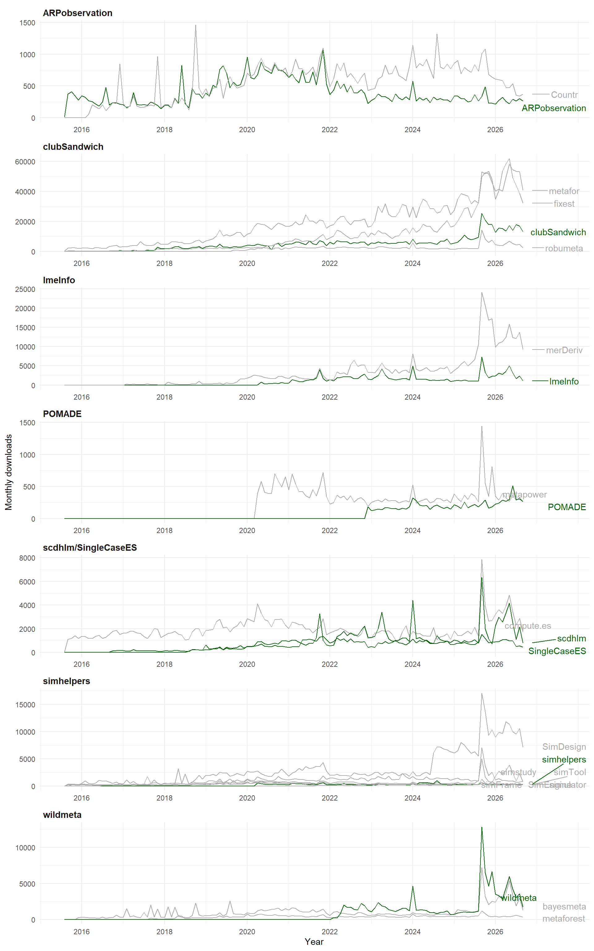
Here are the monthly download rates for each of these packages (note that the vertical scales of the graphs differ):

long_downloads <- 
  readRDS(long_file_name) %>%
  left_join(pkg_groups, by = "package")

long_downloads_select <- 
  long_downloads %>%
  filter(! package %in% c("sandwich","nlme","plm"))

long_downloads_label <- 
  long_downloads_select %>%
  filter(year == 2026, mth == 9) %>%
  mutate(yr = yr + 0.2)

ggplot(long_downloads_select) + 
  aes(yr, count, color = type, group = package, label = package) + 
  geom_line() + 
  geom_text_repel(
    data = long_downloads_label,
    nudge_x = 0.8
  ) + 
  scale_color_manual(values = c(Pusto = "darkgreen", Comparison = "darkgrey")) +
  scale_x_continuous(breaks = seq(2016, 2026, 2)) + 
  expand_limits(y = 0) + 
  expand_limits(x = 2025) + 
  facet_wrap(~ group, scales = "free", ncol = 1) + 
  theme_minimal() + 
  theme(
    legend.position = "none",
    strip.text = element_text(hjust = 0, face = "bold", size = 11)
  ) + 
  labs(
    x = "Year",
    y = "Monthly downloads"
  )